Supernova Progenitor Parameter Estimation with Invertible Neural Networks (INNs)
This is a small (but still interesting) side project I did with INNs. The code I wrote for this project can be found on my GitHub page
Why this matters: Type II supernovae are the violent explosive deaths of massive stars (stars with masses larger than about 8 times of the Sun). Astronomers observe and study their light curves (brightness variation in time) in order to deduce the properties of the underlying exploding stars (so-called supernova progenitors). Knowing the demographics of massive stars can help us better understand how massive stars live and die, how they impact their host galaxies, and how best we should design our future observatories. As in many applications in science, the forward problem of determining measurements given sets of physical parameters is easy. In our case for supernovae, we can perform numerical simulations. However, the inverse problem, that is, inferring the physical parameters given observations is ambiguous. Many sets of parameters can give rise to very similar observables – model degeneracy. For example, in supernova modeling, stars with very different masses and sizes can produce essentially the same light curves. To date, most supernova progenitor parameters are still determined based on visual comparison with incomplete sets of light curve library. To fully characterize the model degeneracy, the posterior parameter distribution conditioned on the observed light curve is required. INN is a recent deep learning architecture designed for reliable posterior estimation. With the imminent deployment of new observatories (e.g. the Vera Rubin Observatory, James Webb Space Telescope), it is timely to explore its applications in real-world scientific settings.
How I approached this: I built an INN for the supernova application using the Framework for Easily Invertible Architecture (FrEIA), a pytorch-based library. The exact INN architecture was rather basic, with three affine coupling blocks of GLOW type interlaced with random permutation layers. The sub-networks in the affine coupling layers were simple fully-connected networks with 3 layers of width 64. The supernova model dataset was taken from my previous published work. Altogether, there were 421 parameters-light curve pairs. Given the relatively small size of the dataset, the size of the INN was also limited (only about 101,000 trainable parameters). My goal was to examine whether such a basic INN is applicable to the supernova inference problem. A total of 337 samples were used in training, while 84 were held out for testing. There are four main physical parameters that determine the supernovae’s observed light curves, namely, the progenitor mass, progenitor radius, explosion energy, and the mass of radioactive nickel.
What I found:
To assess the performance of the INN on our inference problem, we first compare the predicted parameter estimates with the true values. Below we show the scatter plots summarizing the results for two of the key parameters: the explosion energy (\(E_{\rm exp}\)) and the progenitor radius (\(R_{\rm p}\)). The blue crosses denote the predict/true values while the vertical error bars represent the 1-sigma standard deviation of the predictions. The solid black lines show perfect predictions (predicted = true).
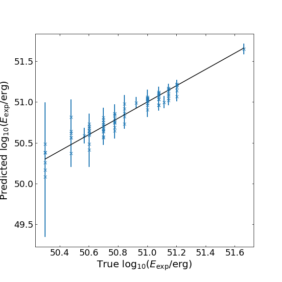
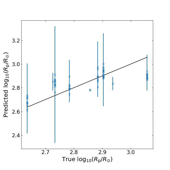
For \(E_{\rm exp}\), the majority of the predictions follows the expected true values. The larger scatter at low energy is expected from the limited data samples in the dataset. For \(R_{\rm p}\), we see that the network is much more uncertain, confirming the known difficulty in predicting the progenitor radius due to model degeneracy.
Next, let’s look at some posterior distributions from selected supernova models.
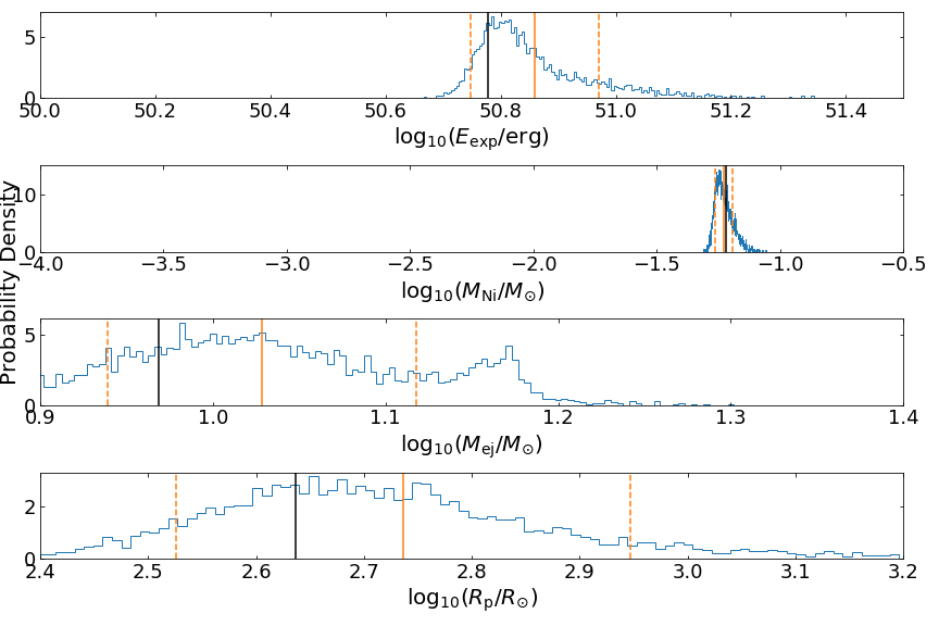
The figure above shows the posterior distributions for a selected test sample predicted by the INN. The blue histograms show the estimated distributions, with orange vertical lines marking the mean value (solid) and 1-sigma range (dashed). The black line in each histogram indicates the true value for the test sample. In this example, the distributions are quite wide and the inferences are uncertain. These histograms capture the correct behavior due to the intrinsic degeneracy in the parameter estimation.
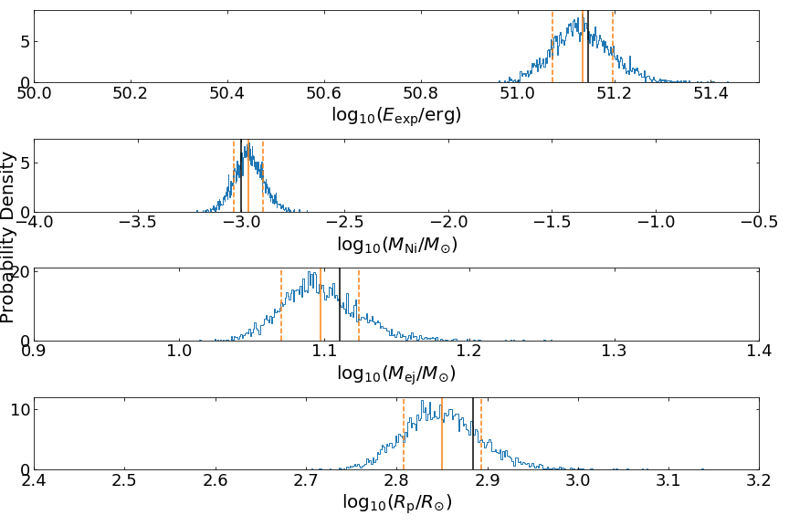
In this next example, the parameters appear to be more well-constrained. It does not mean that we somehow broke the parameter degeneracy. The lack of spread in the posterior distributions is due to the limited number of data samples in this part of the parameter space.
What’s next?
New observatories will soon routinely discover many new supernovae like the ones we modeled above. Having a reliable and readily extendable framework to infer supernovae’s progenitor parameters will be crucial. This exercise demonstrates that INNs can be a powerful and flexible architecture to solve the inverse problem of parameter estimation. Promising directions for future work include expanding the progenitor model library (both in the number of models and physical parameters) and devising ways to incorporate additional prior information (parameter estimates from other observations).